Core functions
Take advantage of Jupyter’s auto-complete functionality (tab key) if you don’t remember a function name or the filename of your data.
You can also (shift+tab+tab) if you don’t remember what a function expects, although sometimes this doesn’t tell you everything (e.g. optional **kwargs to quickPlot)

align
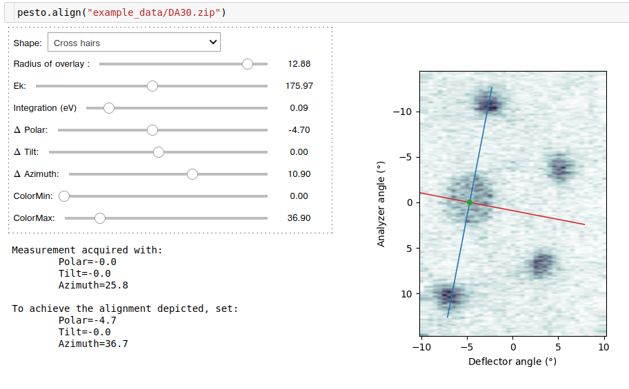
A tool to identify and correct your alignment based on an ARPES map. You will be presented with a constant energy surface, and can adjust the positioning of an overlay. For the default cross-hair overlay, the blue line indicates the analyzer slit. Once the overlay corresponds to the alignment you would like to have, read off the values of polar, tilt and azimuth that are required to achieve it.
def align(spectrum)
Required parameters
spectrum: Path to the data file OR reference to the loaded spectrum object.
Example:
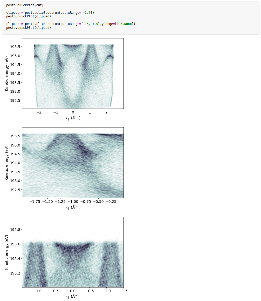
clipSpectrum
Truncates/clips a 1D or 2D spectrum
def clipSpectrum( spectrum,
                  xRange,
                  yRange)
Required parameters
spectrum: The loaded spectrum object to be normalized. Can be of any dimension.
xRange: (optional) 2 element list containing the start and end x values (dimension 1) of the output spectrum, in data units. If they are reversed, the output image will be flipped. If they are left as None or if you provide values outside the range of the spectrum, the maximum/minimum value contained in the spectrum will be used.
yRange: (optional) 2 element list containing the start and end x values (dimension 0) of the output spectrum, in data units. If they are reversed, the output image will be flipped. If they are left as None or if you provide values outside the range of the spectrum, the maximum/minimum value contained in the spectrum will be used. Leave out if you are providing a 1D input scan.
- Returns:
A new spectrum (dictionary object).
Example:
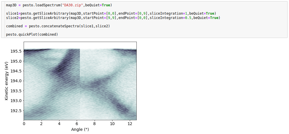
concatenateSpectra
Stitches together two 2D ARPES spectra along the angle or k axis. Intended for the specific case of wanting to combine several images taken at different tilt angles, or slices extracted by pesto.getSliceArbitrary. The concatenation does not consider overlapping regions, so you may need to first trim the input spectra using pesto.clipSpectrum()
def concatenateSpectra(s1,
                      s2)
Required parameters
s1,s2: Loaded spectra
- Returns:
A new spectrum (dictionary object). Note: the angle axis of the output spectrum will always start at zero
Example:
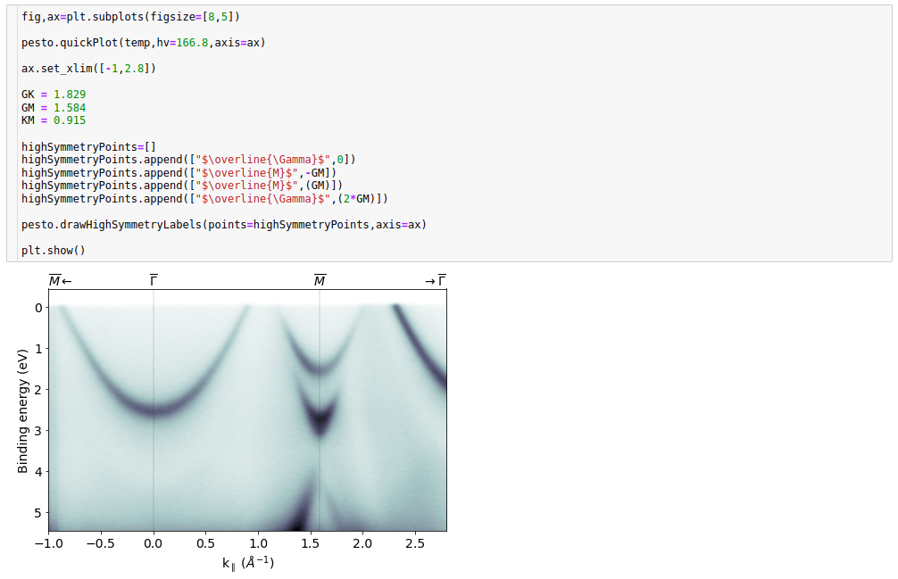
drawHighSymmetryLabels
For drawing high symmetry points on a 2D plot - see the example for clarification.
def drawHighSymmetryLabels( points,
                            axis)
Required parameters
points: A list of high symmetry points to be drawn. Each point is a sub-list containing the string label and the x-axis location - see the example below for clarification
axis: The matplotlib axis object you’d like to label
- Returns:
Nothing (modifies input plot)
Example usage:
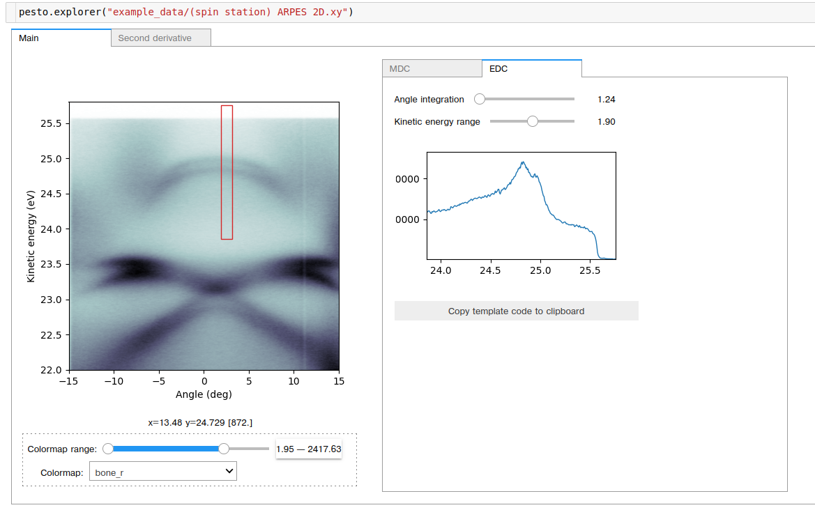
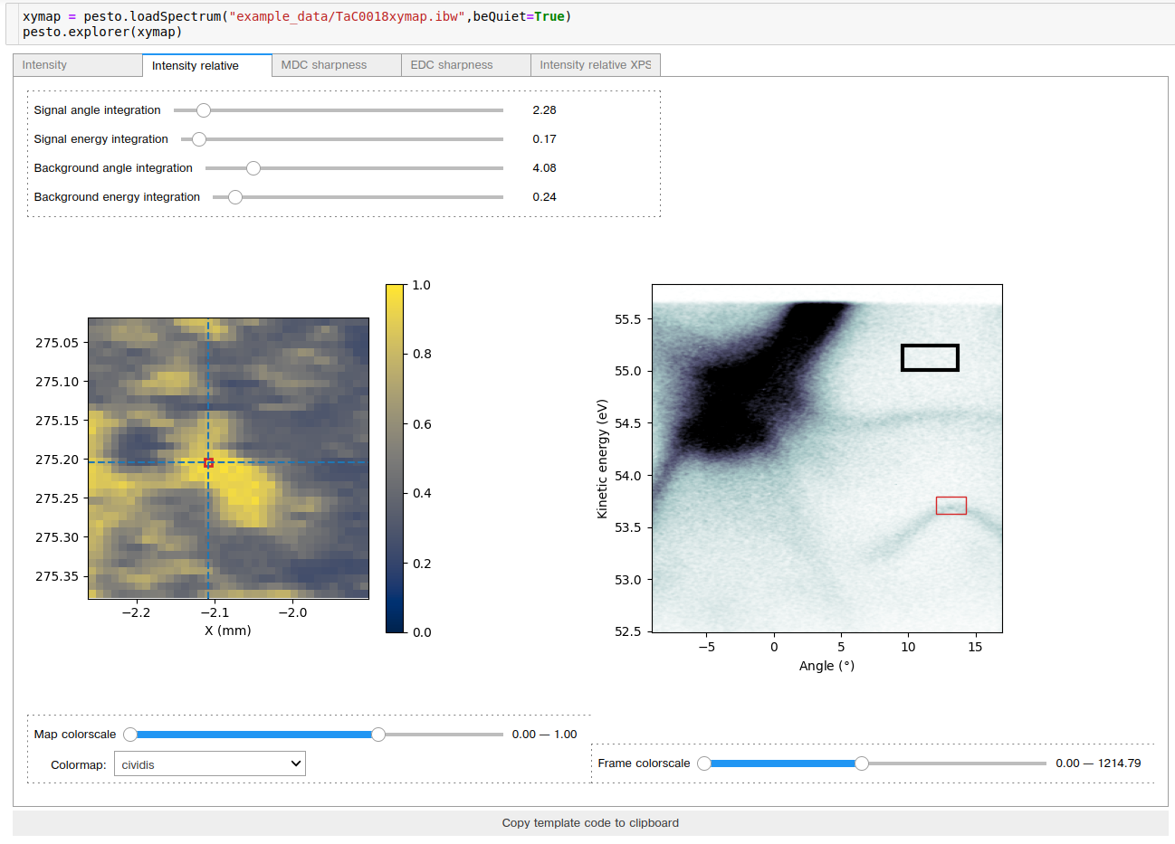
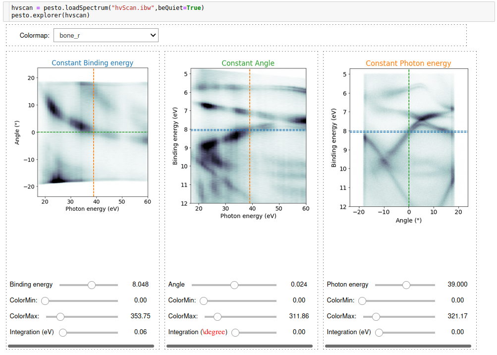
explorer
A general purpose data viewer, capable of interactively showing 2D (ARPES images), 3D (manipulator, deflector, or photon energy scans) or 4D (manipulator raster scan) datasets. It will present whatever data viewer makes the most sense for the spectrum you are giving it.
Some of the explorer interfaces include a ‘Copy template code the clipboard’ button. Pressing this will copy code to the system clipboard, that you can paste into a new cell and run in order to get a static version of whatever is currently showing in the explorer window. This is useful for quickly getting out EDCs or MDCs that span a carefully chosen range, or saving summary images from the spatial map explorer.
def explorer(spectrum)
Required parameters
spectrum: Path to the data file OR reference to the loaded spectrum object.
Examples:
2D ARPES image:
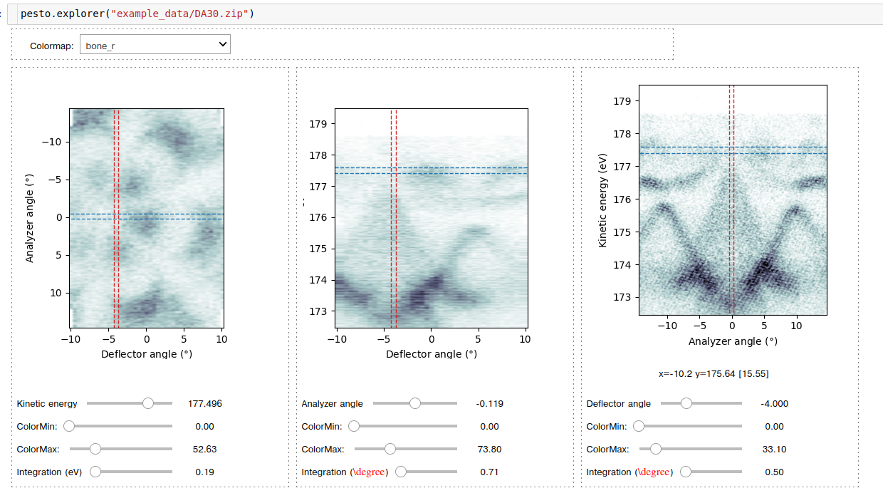
Deflector ARPES scan:
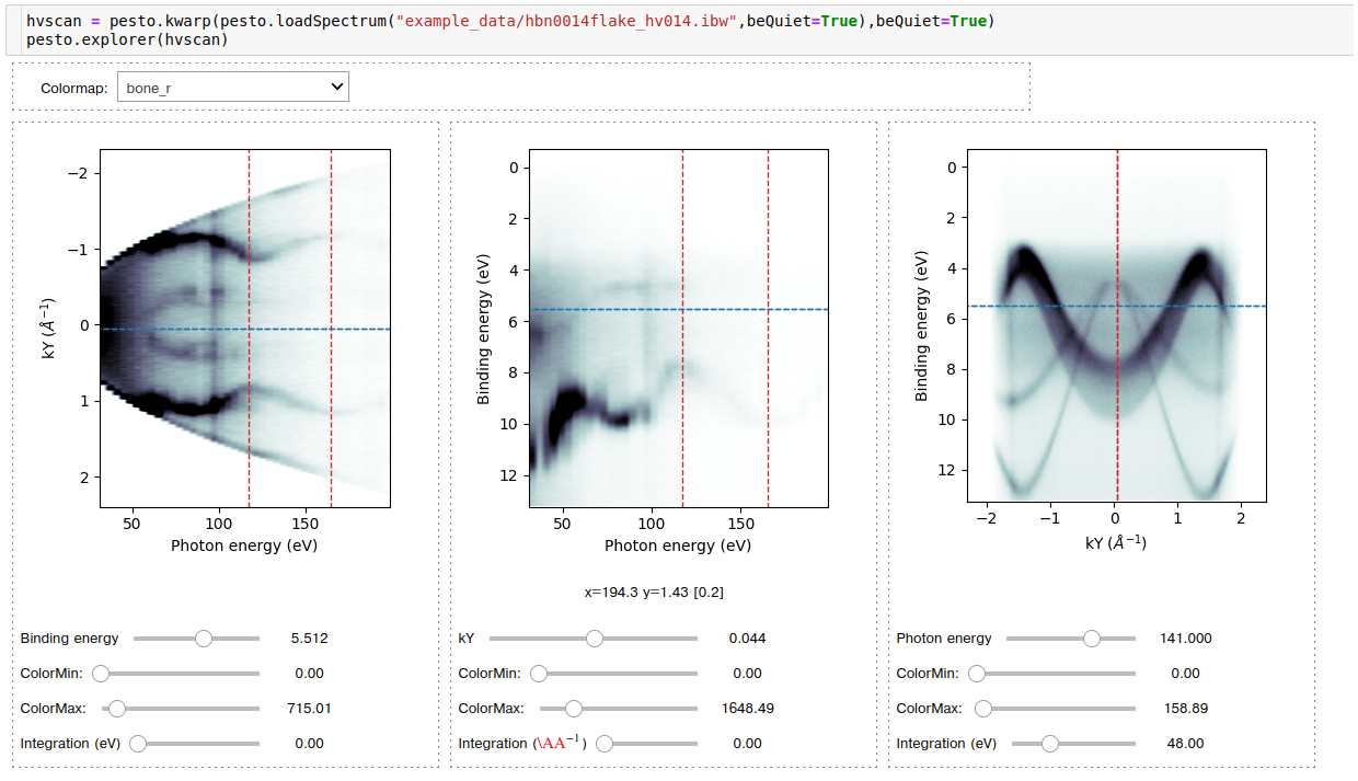
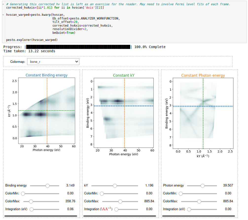
k-warped photon energy scan:
Manipulator X-Y raster scan:
fitFermiEdge
Fits a Fermi edge function to an input spectrum. Leverages the lmfit module to perform the fitting. The base Fermi function used is:
Ef = (1 / (exp((E-Ef)/(kT)) + 1))
Which is then convolved with a Gaussian peak to represent the energy broadening:
Gaussian = exp(-4*log(2)*(E/ResolutionFWHM)^2 )
def fitFermiEdge( spectrum,
                  angleRange,
                  energyRange,
                  linearBG,
                  temperature,
                  beQuiet)
getAnalyzerWorkFunction
Retrieve the internally stored value of the analyzer workfunction.
def getAnalyzerWorkFunction()
Required parameters
none
- Returns
The value of the analyzer workfunction in eV
getFrameFrom4DScan
Extracting a 2D frame from a 4D source spectrum. Intended for use with 2D manipulator scans.
def getFrameFrom4DScan( spectrum,
                        axes,
                        axisValues,
                        beQuiet)
Required parameters
spectrum: The loaded spectrum object to be normalized. Can be of any dimension.
axes: The axes that will be constant in the output 2D frame. Must use the axis label name (e.g. ‘Kinetic energy’, X’ or ‘Angle’), but it will prompt you with your options if you get this wrong. See examples for clarification.
axisValues: Values of the axes (in data units) that should be sampled
beQuiet: If False, prints information about what it’s doing (default = False)
- Returns:
A new spectrum (dictionary object).
Example:

getProfile
Extracts a 1D line profile from a 2D source spectrum
def getProfile( spectrum,
                samplingAxis,
                xAxisRange,
                yAxisRange,
                beQuiet)
Required parameters
spectrum: The loaded spectrum object to extract a line profile from. Data field must be 2D.
samplingAxis: Which direction to sample (‘x’ (dimension 1) or ‘y’ (dimension 0)). On an E-k image, ‘x’ –> MDC, ‘y’ –> EDC
Optional parameters
xAxisRange: X axis range, in data units - if samplingAxis were ‘x’, this would be the span of the profile. If samplingAxis were ‘y’, this would be the integration level. A value of ‘None’ means ‘don’t care’, so e.g. samplingAxis=’x’ with xAxisRange=[None,None] would cover the entire x-axis of the input spectrum. Default = [None,None]
yAxisRange: Y axis range, in data units. Same comments apply as for xAxisRange. Default = [None,None]
beQuiet: If False, prints information about what it’s doing (default = False)
- Returns:
A new spectrum (dictionary object) containing the 1D line profile
getProfileArbitrary
Extracts a 1D line profile from a 2D source spectrum, along an arbitrary direction.
def getProfileArbitrary( spectrum,
                startPoint,
                endPoint,
                sliceIntegration,
                beQuiet)
Required parameters
spectrum: The loaded spectrum object to extract a line profile from. Data field must be 2D, and must have the same units on both axes
startPoint: The [x,y] coordinates in data units where the profile should start (e.g. [-5.1,2.2])
endPoint: The [x,y] coordinates in data units where the profile should end
Optional parameters
sliceIntegration: Integration along the normal axis of the profile, in data units. Default = 0 (no integration)
beQuiet: If False, prints information about what it’s doing (default = False)
- Returns:
A new spectrum (dictionary object) containing the 1D line profile
Example:

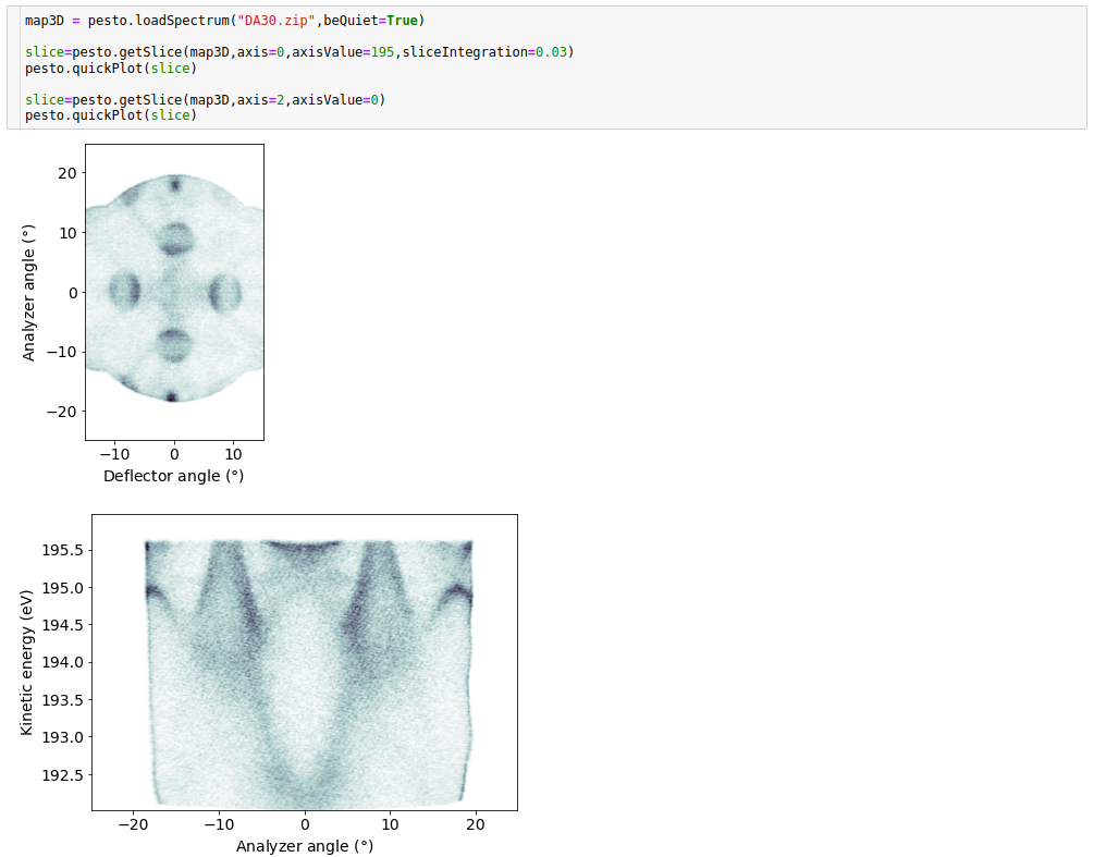
getSlice
The simple version of extracting a 2D slice from a 3D source spectrum. Constrained to taking a slice aligned with one of the source axes (i.e. constant x,y or z slice)
def getSlice( spectrum,
              axis,
              axisValue,
              sliceIntegration,
              normalized,
              beQuiet)
Required parameters
spectrum: The pesto spectrum object to extract a line profile from. Data field must be 3D (e.g. photon energy scan, manipulator polar scan, deflector map).
axis: Which axis the slice should be taken from. Valid options are [0,1,2]. By convention within pesto, axis 0 is the energy axis, axis 1 is the analyzer angle axis and axis 2 is whatever the third dimension was (e.g. polar angle, photon energy…)
axisValue: Where the slice should be taken, in data units. E.g. axis=0,axisValue=44 would yield a constant energy surface at 44eV.
Optional parameters
sliceIntegration: Integration along the normal axis of the slice, in data units. Default = 0 (no integration)
normalized: If True, the intensity within the data slice will be rescaled as you change sliceIntegration. This is mainly here for the interactive explorer functions, to avoid needing to adjust the color scale when you change the slice integration. Default = False
beQuiet: If False, prints information about what it’s doing (default = False)
- Returns:
A new spectrum (dictionary object)
Example:
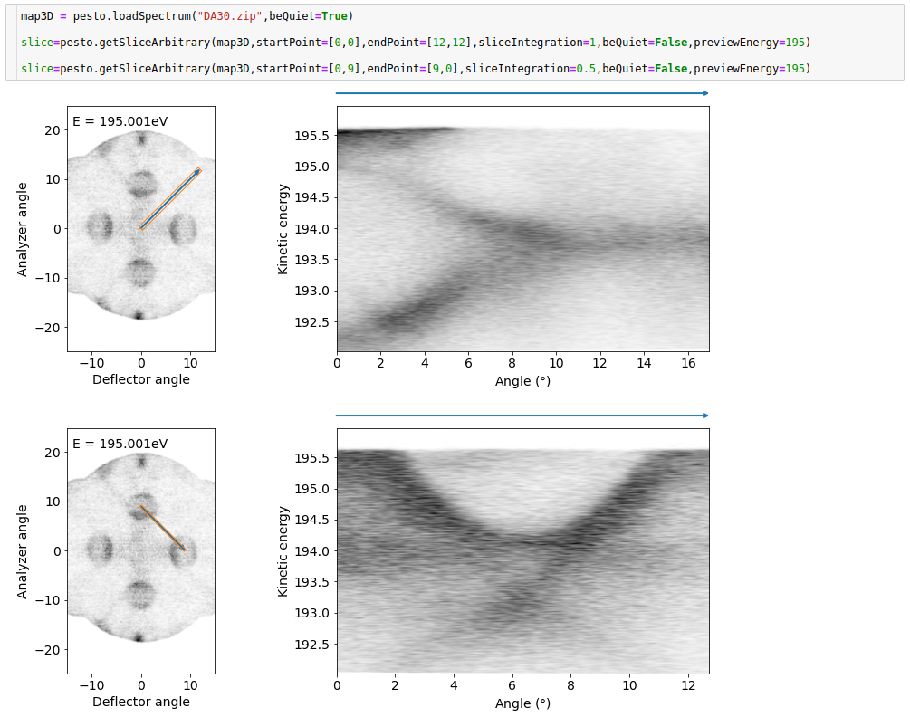
getSliceArbitrary
Extracts a 2D slice from a 3D ARPES spectrum (i.e. energy-angle-angle), along an arbitrary line on a constant energy surface (see examples for clarification. Intended for extracting high-symmetry cuts from a Fermi surface map.
def getSlice_arbitrary( spectrum,
                        startPoint,
                        endPoint,
                        sliceIntegration,
                        beQuiet,
                        previewEnergy)
Required parameters
spectrum: The loaded spectrum object to extract a slice from. Data field must be 3D, and must have axes of energy-angle-angle or energy-k-k
startPoint: A two element list with the x- and y- components, in data units, of the start of the slice path
endPoint: A two element list with the x- and y- components, in data units, of the end of the slice path
Optional parameters
sliceIntegration: Integration in the direction normal to the slice, in data units. Default = 0 (no integration)
beQuiet: If False, prints a two-panel plot. The left panel is a constant energy surface indication where the slice is being taken (blue line) and the integration level (orange box). The right panel contains the extracted slice. Default = False
previewEnergy: The energy value for the constant energy slice shown in the preview if beQuiet=False. Default = 0, which will probably correspond the lowest energy slice
- Returns:
A new spectrum (dictionary object). Note: the angle axis of the output slice will always start at zero
Example:
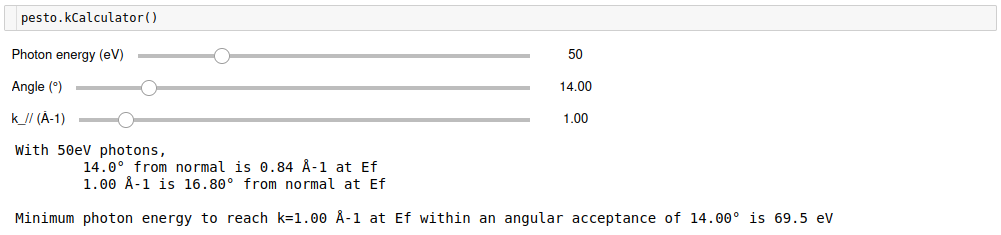
kCalculator
An interactive calculator for mapping between angle values and k values.
def kCalculator()
Example:
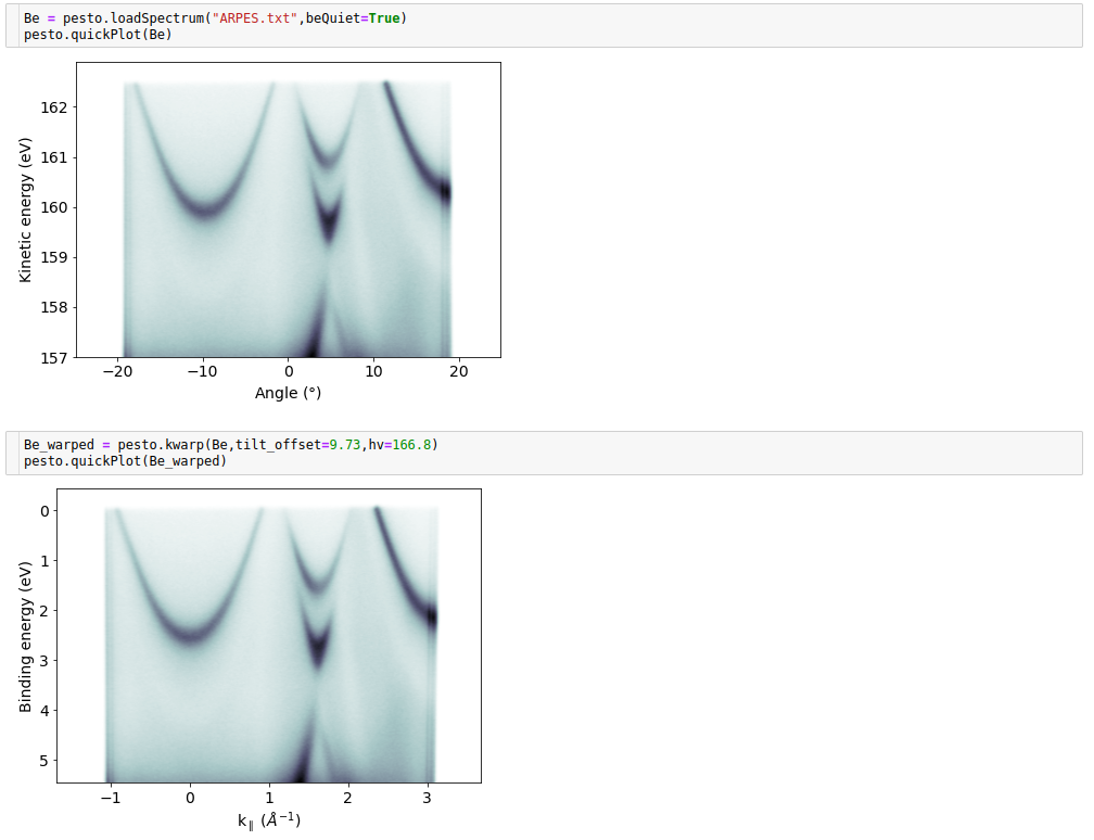
kwarp
Transform an input spectrum from angle space to k-space.
def kwarp(  spectrum,
            Eb_offset,
            corrected_hvAxis,
            polar_offset,
            tilt_offset,
            hv,
            resolutionDivider
            beQuiet)
Required parameters
spectrum: The loaded spectrum object to be k-warped. Valid inputs are 2D energy-angle images, 3D manipulator scans, 3D deflector maps and 3D photon energy scans. Photon energy scans must have the energy axis as binding energy, all other types must have the energy axis as kinetic energy. Photon energy scans are only k-warped for parallel momentum, not k_z.
Optional parameters
Eb_offset: When k-warping photon energy scans, pesto will convert each frame back to kinetic energy based on the analyzer workfuntion and the photon energy. However SES calculates the binding energy scale assuming a work function of 0, so there is usually a binding energy offset equal to the analyzer workfunction (i.e. Ef appears at Eb=4.5eV). Select a different offset with this parameter if required. Default = whatever the global ANALYZER_WORKFUNCTION parameter is set to.
corrected_hvAxis: If the monochromator calibration is not perfect, you may pass in a list consisting of the corrected photon energy axis. This will take care of aligning all frames in binding energy. See examples below for clarification. Default = [] (empty list)
polar_offset: What offset to apply to the polar angle in the spectrum in order to make a polar angle of zero correspond to normal emission. For example, if normal emission is at polar angle=+8.2 in the spectrum, you would pass in a polar offset of -8.2. Not applicable for k-warping photon energy scans, which will always assume a zero polar offset. Default = 0
tilt_offset: What offset to apply to the analyzer angle in the spectrum in order to make zero on the analyzer slit axis correspond to normal emission. For example, if normal emission located at angle=-5.3 in the spectrum, you would pass in a tilt offset of +5.3. Default = 0
hv: If you pass in a photon energy, the output will be in binding energy instead of kinetic energy. Does not apply to photon energy scans. Default = 0, which means do nothing.
resolutionDivider: Divide down the resolution of the output spectrum in all dimensions by an integer factor - useful if you need it to go faster. Default = 1 (i.e. no adjustment)
beQuiet: If False, prints information about what it’s doing (default = False)
- Returns:
A new spectrum (dictionary object)
Example:
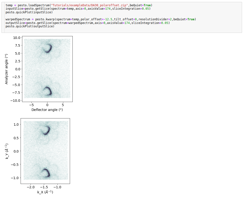
The next example is from a 3D deflector map dataset taken on graphene with K-M-K alignment, so a large polar offset is needed. Here we display 2D constant energy slices before and after the kwarp.
The final example is from a photon energy scan dataset, acquired at a large tilt angle. In the original spectrum the miscalibration of the photon energy manifests as a sloping Fermi level, and we correct for this during the k-warp.
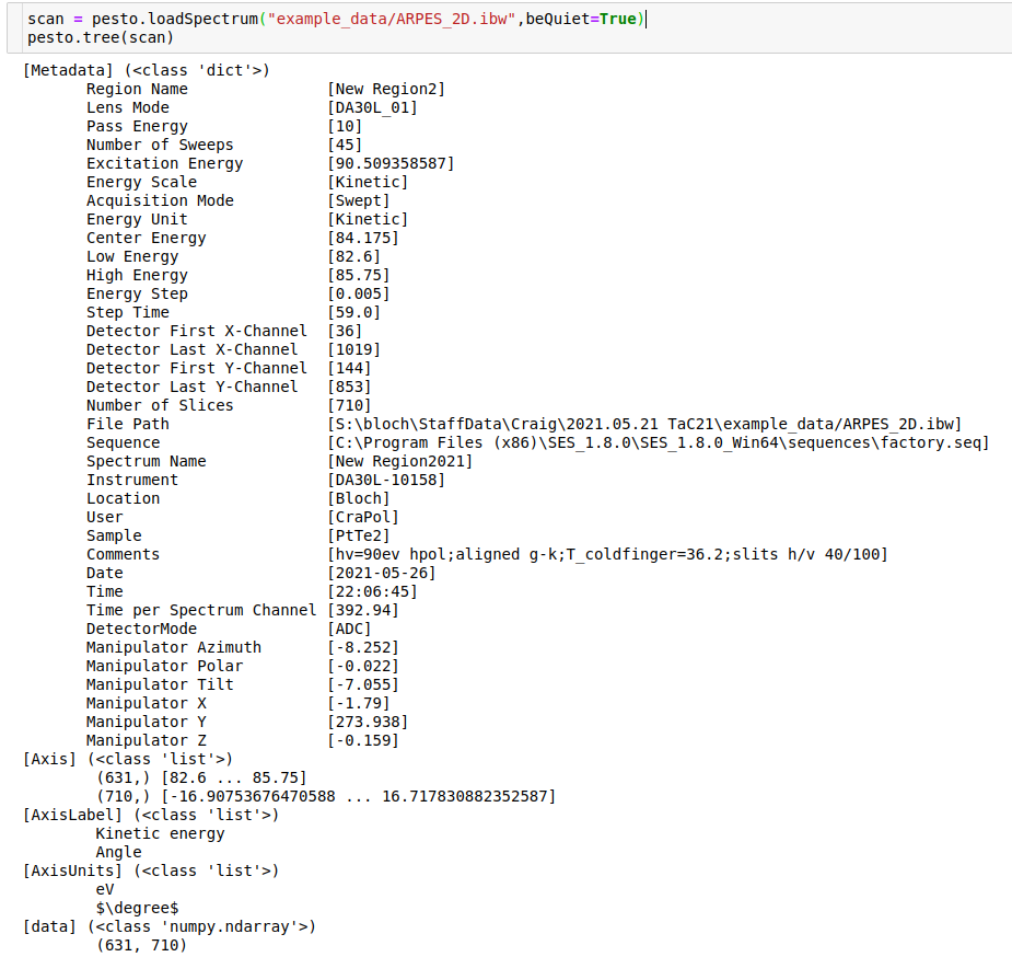
loadSpectrum
The loadSpectrum function reads a saved data file, tries to infer what kind of measurement it is and then returns a dictionary object containing the data, axis information and metadata. Pesto calls this dictionary object a ‘spectrum’, and most other pesto functions take one of these as input.
The inferences and metadata typically rely on quirks of how data is saved in the specific installations that are supported, i.e. modifications will probably be needed for measurements taken elsewhere.
The procedures for loading each supported file type can be found under pesto/fileLoaders.
def loadSpectrum(spectrum)
Required parameters
fileName: Path to the file you want to load. Currently supports sp2,itx,xy,txt,ibw,sr and zip files from Bloch and the older i3/i4 beamlines of Max IV.
- Optional parameters:
beQuiet: If False, prints information about what it’s doing (default = False)regionIndex: If this is a multi-region zip file from SES, specify which region index you want to load. Default = 1whichManipulatorAxis: If multiple axes were scanned in a nominally 1D manipulator scan, specify which one should be considered the major axis. Default = ‘’ (i.e. none specified)mask: Specific to spin datasets, this will allow you to ignore (‘mask off’) specified coilPolarity steps in the dataset. Provide a list the same length as the number of coil polarity steps. Any element set to zero means ‘don’t load this step’. For example, mask=[1,1,0,1,1,1,1,1] means drop the third scan in the series. Default = [] (empty list, no masking)- Returns:
A pesto ‘spectrum’ (Dictionary object)
Example usage:

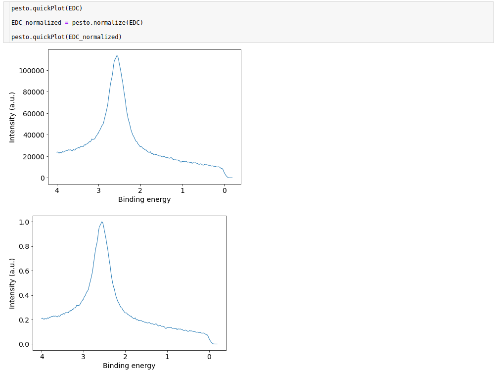
normalize
Simple normalization of the data field of a spectrum - first subtracting the minimum value then dividing by the maximum value.
def normalize(spectrum):
Required parameters
spectrum: The loaded spectrum object to be normalized. Can be of any dimension.
- Returns:
A new spectrum (dictionary object).
Example:
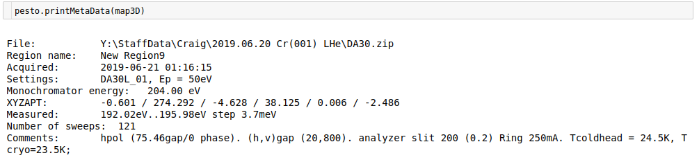
printMetaData
Prints a metadata summary of a loaded spectrum (the same information that is by default shown when calling pesto.loadSpectrum)
def printMetaData(spectrum):
- Returns:
Nothing (prints to console)
Example:
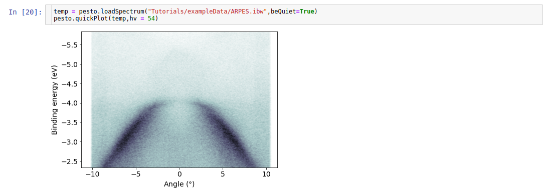
quickPlot
quickPlot is a means of quickly throwing up a plot of 1D or 2D data. It’s possible but not required to use this with other matplotlib functions if you’d like to adjust the presentation of the figure.
def quickPlot(spectrum,
              hv,
              axis,
              label,
              cmap,
              cmin,
              cmax,
              lw,
              color,
              logscale,
              XPS,
              returnIm,
              spinProjection,
              filled,
              alpha,
              kPath,
              nkpnts,
              drawHighSymmetryLabels,
              bandIndicesToPlot,
              Eb,
              errorbars,
              fillToZero,
              alpha,
              beQuiet)
- Required parameters
spectrum: Name of the loaded spectrum OR path to the datafile that you want to plot.
Optional parameters
hv: If you pass in a photon energy, the plot will be in binding energy instead of kinetic energy. Default = None, meaning don’t convert to binding energy.
axis: If you pass in a matplotlib axis, quickPlot will put the plot there instead of making a new figure. Used when you want to be able to adjust the plot afterwards, and/or when you want repeated calls to quickPlot to draw all traces on the same plot. Default = None (meaning create a new figure and plot there)
label: For 1D traces, attach a label for a matplotlib legend to use. Default = None
cmap: For 2D image plots, specify the colormap to use. (options.). Default = ‘bone_r’
cmin: For 2D image plots, specify the minimum data value the colormap covers. Default = False, meaning use the maximum data value
cmax: For 2D image plots, specify the maximum data value the colormap covers. Default = None, meaning use the minimum data value
lw: For 1D traces, linewidth to use. Default=1
color: For 1D traces, color to use (options.) Default = None (meaning it cycles through the default matplotlib colors). If using the ‘filled’ option, the color should be explicity named, otherwise the line and fill will not match.
logscale: For 1D traces, if True then plot with a log y-axis. For 2D images, if True then plot the log of the input data. Default = False
XPS: For 2D image inputs: if True, collapse all angles to turn it into a 1D dataset, then plot that. Default = False
returnIm: If true, pass back the return value of the matplotlib pyplot call. Primarily used internally by the interactive data explorers. Default = False
errorbars: For 1D plots, if set to True AND the input spectrum contains the error bars values in an [‘errorbars’] entry, then they will be included in the plot. Default = False, meaning don’t plot error bars.
spinProjection: For DFT slab bandstructure. If 0, 1 or 2 then plot the spin projection on the x, y or z axis respectively. Assumes that the spin projection information exists within the spectrum loaded. Default = None, meaning don’t try to plot spin.
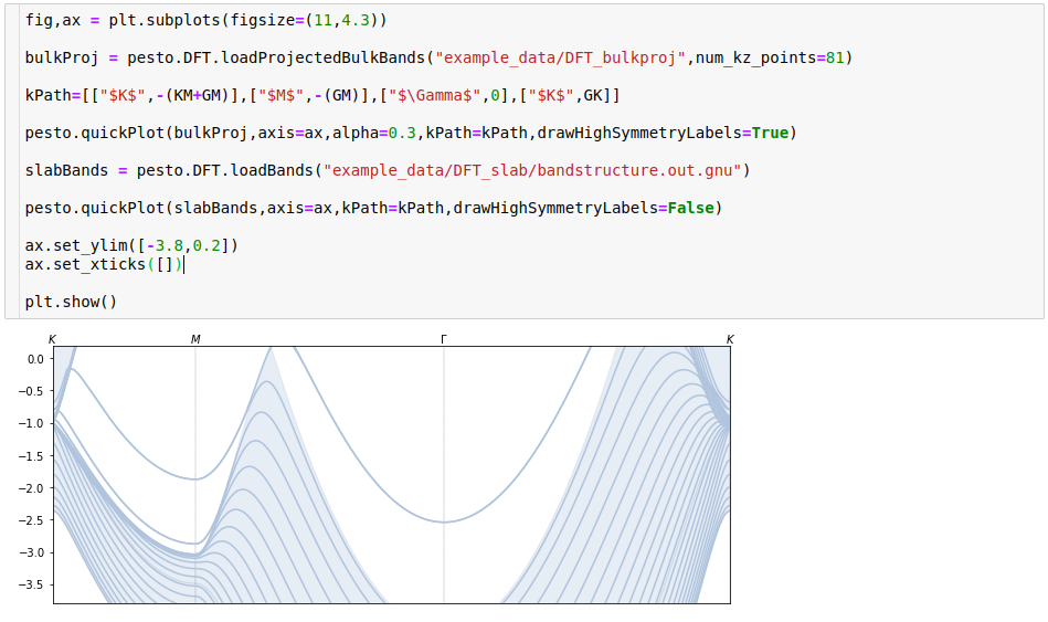
filled: For 1D profiles, if True the plot will be filled to zero. For DFT projected bulk bandstructure plots, if True the different kz values will be rendered as a solid region rather than individual bands. Default = True for DFT plots, False for 1D profiles.
alpha: If filled=True, OR if errorbars=True, choose the transparency (alpha value) of the shading. 1 = no transparency, 0 = fully transparent. Default = 1 for DFT plots, 0.1 for 1D profiles.
kPath: For DFT plots, to set the k-axis correctly. Pass in K point labels and positions as a list, for example kPath=[[“$M$”,-1.1],[“$Gamma$”,0]]. The number of points in the list must match that of the kpath used in the calculation. See examples for clarification. Default=None, meaning just use a linearly increasing k-axis starting from zero.
drawHighSymmetryLabels: For DFT plots. If True, annotate the plot with high symmetry labels according to the kPath you provided (if you provided one). Default = False
bandIndicesToPlot: For DFT slab bandstructure. Provide a list of band indexes to plot, hide all others. Default = None, meaning plot all bands.
beQuiet: If False, prints information about what it’s doing. Default = False
- Returns:
Nothing (draws a plot)
Example usage:
If you just want a preview, it’s a one-liner:
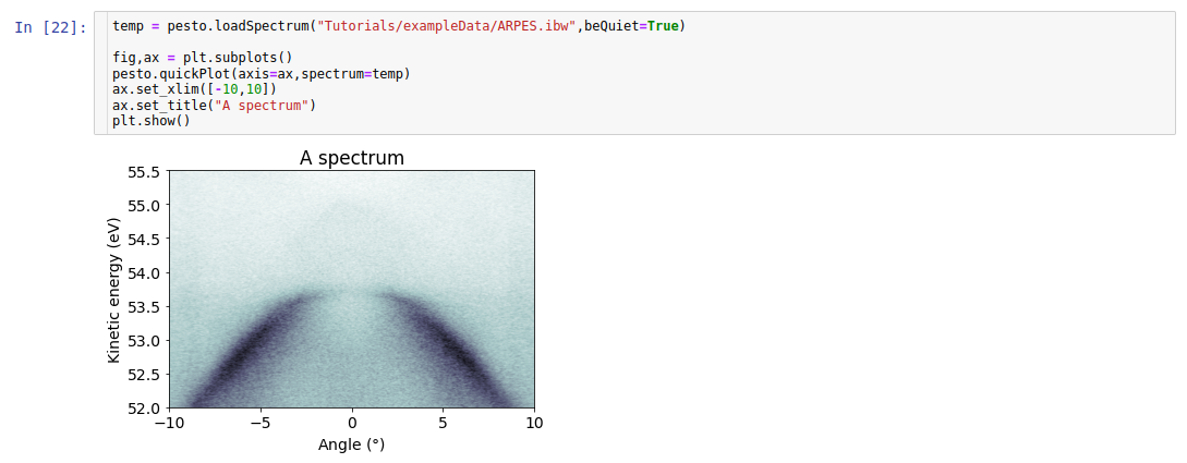
But you can also pass in a matplotlib axis object for it to use. The advantage of this approach is that you can change the styling, size, labels etc:
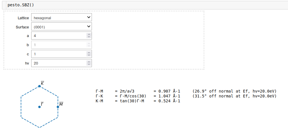
SBZ
An interactive calculator for the surface brillouin zone size, given a lattice type and size. Zone projection images are based on the figures in Lüth, ‘Solid Surfaces, Interfaces and Thin Films’, 6th ed, p224-226.
def SBZ()
Example:
setAnalyzerWorkFunction
Update the internally stored value of the analyzer workfunction, which is used by various other functions such as quickPlot or fitFermiEdge. Use it if the value has changed between datasets or the default value does not apply to your dataset. The change only persists within that notebook environment.
def setAnalyzerWorkFunction(value)
Required parameters
value: The analyzer workfunction in eV. The default value is printed when you import pesto.
- Returns
Nothing
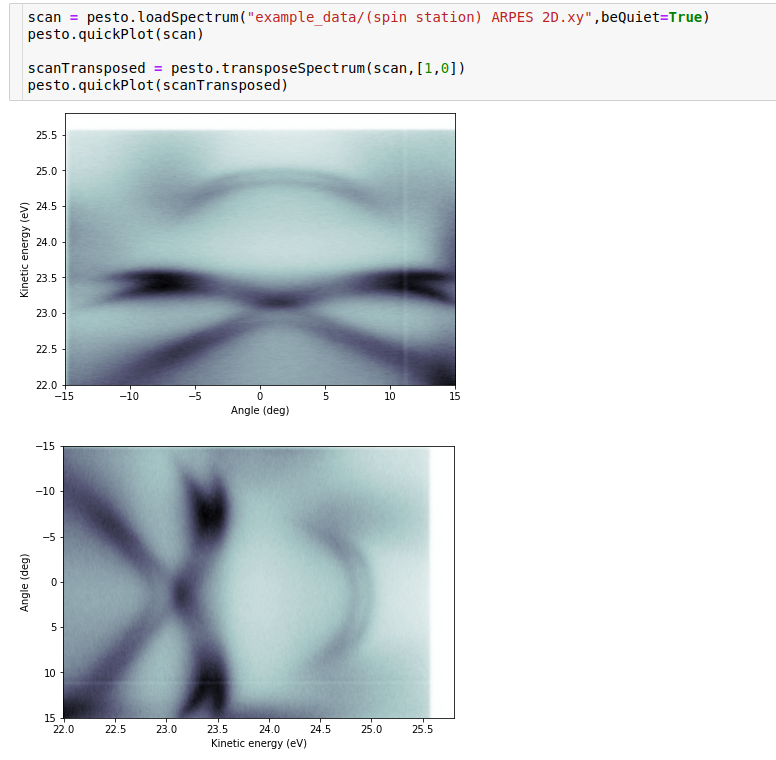
transposeSpectrum
A wrapper for numpy’s transpose function that will simultaneously shift around the axes. Allows you to, for example, swap the angle and energy axes in a spectrum.
def transposeSpectrum(spectrum,a)
Required parameters
spectrum: A pesto ‘spectrum’
a: A list of what the new ordering should be. For example, if the input data were a 3D matrix, a = [1,3,2] would swap the first and last dimensions.
- Returns
A new spectrum (dictionary object) with the re-ordered axes.
Example:
tree
Prints an overview of the contents of a spectrum object.
def tree(spectrum)
Required parameters
spectrum: A pesto ‘spectrum’
- Returns
Nothing (prints to console)
Example: