Code snippets and examples
Useful code blocks to copy+paste
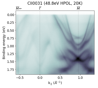
Labelled, kwarped E-k image
Here we load a 2D image, kwarp it (correcting for a tilt offset) and then plot it. The pesto function drawHighSymmetryLabels handles the high symmetry
GM,GX = 0.952,0.673
hv = 48.75

scan = pesto.loadSpectrum("CII0031.ibw",beQuiet=True)
scan = pesto.kwarp(scan,tilt_offset=7.2)

fig,ax=plt.subplots(figsize=(6,5))
ax.set_title("CII0031 ({:.1f}eV HPOL, 20K)".format(hv),y=1.07)
pesto.quickPlot(scan,axis=ax,hv=hv)
ax.set_xlim([-0.6,1.35])
highSymmetryPoints=[[r"$\overline{\Gamma}$",0],[r"$\overline{M}$",GM],[r"$\overline{M}$",-GM]]
pesto.drawHighSymmetryLabels(points=highSymmetryPoints,axis=ax)
plt.show()
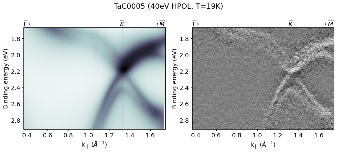
E-k image next to its second derivative
The easiest way to generate the code for the second derivative plot (and to know what filtering and colorscale settings to use) is to first compose the image in pesto.explorer(), then use the “Copy template code to clipboard” button.
import scipy,copy

GK=1.326
GM=1.148
KM=0.663

scan = pesto.kwarp(pesto.loadSpectrum("snippets/TaC0005New Region1005.ibw",beQuiet=True),tilt_offset=21.5,polar_offset=0,beQuiet=True)
hv = 40

fig,axes=plt.subplots(figsize=(11,5),ncols=2)
plt.suptitle("TaC0005 ({}eV HPOL, T=19K)".format(hv))

ax=axes[0]
pesto.quickPlot(scan,axis=ax,hv=hv)
highSymmetryPoints=[["$\overline{\Gamma}$",0],["$\overline{K}$",GK],["$\overline{M}$",GK+KM]]
pesto.drawHighSymmetryLabels(points=highSymmetryPoints,axis=ax)

ax=axes[1]
tempSpectrum=copy.deepcopy(scan)
tempSpectrum['data']=scipy.ndimage.uniform_filter1d(tempSpectrum['data'], 14, 0) #
tempSpectrum['data'] = np.diff(tempSpectrum['data'], n=2,axis=0)
pesto.quickPlot(tempSpectrum,axis=ax,hv=hv,cmax=25,cmin=-25,cmap='gray_r')
pesto.drawHighSymmetryLabels(points=highSymmetryPoints,axis=ax)

plt.tight_layout()
plt.show()
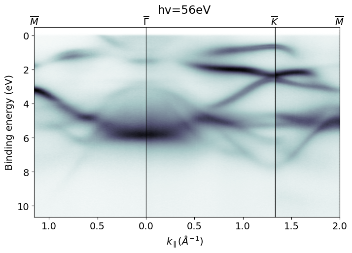
Stacking several images taken at different tilt/azimuths
Here we have acquired a series of images to obtain a cut along the high symmetry path M-G-K-M.
GK,GM,KM =1.331, 1.153, 0.666

GM_scan=pesto.kwarp(pesto.loadSpectrum("TaC_0086Valence bands shallow.ibw", beQuiet=True),tilt_offset=10)
GK_scan=pesto.kwarp(pesto.loadSpectrum("TaC_0081Valence bands shallow.ibw", beQuiet=True),tilt_offset=10)
KM_scan=pesto.kwarp(pesto.loadSpectrum("TaC_0078Valence bands shallow.ibw", beQuiet=True),tilt_offset=25)
hv=56

fig = plt.figure(figsize=(8,5))
gs = matplotlib.gridspec.GridSpec(1, 3, width_ratios=[GM,GK,KM], height_ratios=[1])
gs.update(wspace = 0, hspace = 0)

ax = fig.add_subplot(gs[0])
GM_cropped=pesto.clipSpectrum(GM_scan,xRange=[0,GM])
pesto.quickPlot(GM_cropped,axis=ax,hv=hv)
highSymmetryPoints=[["$\overline{M}$",GM]]
pesto.drawHighSymmetryLabels(points=highSymmetryPoints,axis=ax)

ax.set_xticks([0.50,1.0]) # Customize the x-ticks
ax.set_xlim([GM,0]) # Reverse the x-axis
ax.set_ylim([None,-0.5])
ax.set_xlabel("")

ax = fig.add_subplot(gs[1])
GK_cropped=pesto.clipSpectrum(GK_scan,xRange=[0,GK])
pesto.quickPlot(GK_cropped,axis=ax,hv=hv)
highSymmetryPoints=[["$\overline{\Gamma}$",0],["$\overline{K}$",GK]]
pesto.drawHighSymmetryLabels(points=highSymmetryPoints,axis=ax)
ax.set_ylabel("")
ax.set_xlabel('$k_\parallel (\AA^{-1})$', x=0.3)
ax.set_yticks([])
ax.set_ylim([None,-0.5])
ax.set_title("hv=56eV",y=1.05,x=0.3)

ax = fig.add_subplot(gs[2])
KM_cropped=pesto.clipSpectrum(KM_scan,xRange=[GK,GK+KM])
pesto.quickPlot(KM_cropped,axis=ax,hv=hv)
highSymmetryPoints=[["$\overline{M}$",GK+KM]]
pesto.drawHighSymmetryLabels(points=highSymmetryPoints,axis=ax)
ax.set_ylabel("")
ax.set_xlabel("")
ax.set_yticks([])
ax.set_ylim([None,-0.5])
ax.set_xlim([None,2])

plt.show()
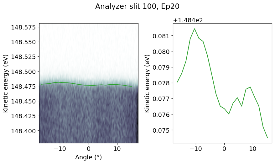
Quantifying Fermi edge warping
All analyzer slits at Bloch are straight, and consequently produce curved Fermi levels as seen on the raw detector image. Built-in curvature correction straightens the image, but sometimes this is not perfect or some other effect might cause warping. Here is an example of characterizing the distortion by automatically fitting a series of EDCs through the Fermi level.
scan = pesto.loadSpectrum("Au0002Au002.ibw",beQuiet=True)

angleBin = 1.5
angleRange = scan['Axis'][1][-1]-scan['Axis'][1][0]
anglesToSample = [scan['Axis'][1][0]+(angleBin/2) + ii*angleBin for ii in range(int(angleRange/angleBin))]

fermiLevel = []
for angle in anglesToSample:
    params = pesto.fitFermiEdge(spectrum=scan,angleRange=[angle-angleBin/2,angle+angleBin/2],energyRange=[148.39,148.56],linearBG=True,temperature=20,beQuiet=True)
    fermiLevel.append(params['FermiLevel'].value)

fig,axes=plt.subplots(figsize=[9,5],ncols=2)

ax=axes[0]
pesto.quickPlot(scan,axis=ax)
ax.plot(anglesToSample,fermiLevel,color='tab:green')

ax=axes[1]
ax.plot(anglesToSample,fermiLevel,color='tab:green')
ax.set_ylabel("Kinetic energy (eV)")

plt.tight_layout()
plt.suptitle("Analyzer slit 100, Ep20",y=1.05)
plt.show()
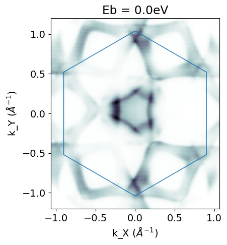
Constant energy surfaces with Brillouin zone overlay
fig,ax = plt.subplots(figsize=(5,5))

PT2_22 = pesto.kwarp(pesto.loadSpectrum("snippets/PtTe20022.zip",beQuiet=True),beQuiet=True)

Ef = 89.9-pesto.ANALYZER_WORKFUNCTION
GK=1.041
Eb = 0

ax.add_patch(matplotlib.patches.RegularPolygon((0,0), numVertices=6, radius=GK, orientation=math.radians(0),linestyle='-',color='tab:blue',fill=False,lw=1))
slice = pesto.getSlice(spectrum=scan_kwarped,axis=0,axisValue=Ef-Eb,sliceIntegration=0.03,normalized=True)
pesto.quickPlot(slice,axis=ax)
ax.set_ylim([-1.2,1.2])
ax.set_title("Eb = {:.1f}eV".format(Eb))

plt.show()
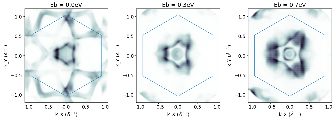
Or if you want several cuts side by side:
fig,axes = plt.subplots(figsize=(14,5),ncols=3)

PT2_22 = pesto.kwarp(pesto.loadSpectrum("snippets/PtTe20022.zip",beQuiet=True),beQuiet=True)

Ef = 89.9-pesto.ANALYZER_WORKFUNCTION
GK=1.041
Eb = 0

for index,Eb in enumerate([0.0,0.35,0.7]): #Specify which Eb cuts we want
                ax=axes[index]
                ax.add_patch(matplotlib.patches.RegularPolygon((0,0), numVertices=6, radius=GK, orientation=math.radians(0),linestyle='-',color='tab:blue',fill=False,lw=1))
                slice = pesto.getSlice(spectrum=scan_kwarped,axis=0,axisValue=Ef-Eb,sliceIntegration=0.03,normalized=True)
                pesto.quickPlot(slice,axis=ax)
                ax.set_ylim([-1.2,1.2])
                ax.set_title("Eb = {:.1f}eV".format(Eb))

plt.tight_layout()
plt.show()
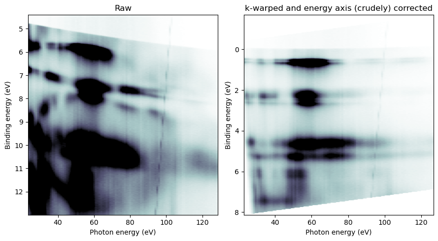
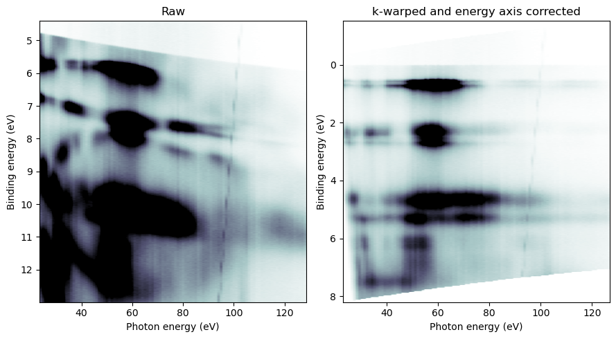
Correcting monochromator energy calibration in hv-sweeps
Sometimes the monochromator energy calibration is off, and it can be a headache to visualize photon energy scans. If you know how the energy calibration is off, you can pass in a corrected photon energy axis when k-warping the dataset.
If a simple linear correction will suffice, you would do something like this (trial-and-error to find the linear coefficients):
hvscan = pesto.loadSpectrum(dataPath+"TaC0027New Region7.ibw",beQuiet=True)

corrected_hvAxis = [hv*0.988 - 0.23 for ii,hv in enumerate(hvscan['Axis'][2])] #You should iteratively tweak the scaling factor as needed

hvscan_kwarped = pesto.kwarp(hvscan,
                             Eb_offset = pesto.getAnalyzerWorkFunction(),
                             corrected_hvAxis=corrected_hvAxis,
                             tilt_offset=22,
                             resolutionDivider=3,
                             beQuiet=False)

 #------- Plot the result
fig,axes = matplotlib.pyplot.subplots(figsize=(9,5),ncols=2)

ax=axes[0]
axisValue,integration = 0,3
slice=pesto.getSlice(hvscan,axis=1,axisValue=axisValue,normalized=True,sliceIntegration=integration,beQuiet=True)
pesto.quickPlot(slice,axis=ax,cmin=0.00,cmax=250,cmap='bone_r')
ax.set_title("Raw")

axisValue,integration = 1.362,0.167
ax=axes[1]
slice=pesto.getSlice(hvscan_kwarped,axis=1,axisValue=axisValue,normalized=True,sliceIntegration=integration,beQuiet=True)
pesto.quickPlot(slice,axis=ax,cmin=0.00,cmax=550,cmap='bone_r')
ax.set_title("k-warped and energy axis (crudely) corrected")
plt.tight_layout()
plt.show()
If you need something a little more exact, and if your measurements support fitting a Fermi edge on every frame, here is an example of a more sophisticated approach:
#hvscan = pesto.loadSpectrum(dataPath+"TaC0027New Region7.ibw",beQuiet=True)

#------- One possible approach to extracting the Fermi edge position frame-by-frame.
# How you solve this will depend on what your spectra look like at Ef

width=0.13 # Width either side of Ef that the fit will use during the first pass
width_fine=0.08 #Smaller window on the second pass
angleRange=[-15,15] #Angle range that the fit will use
temperature = 77
corrected_hv_axis = []
beQuiet=True # Set this to False in order to inspect each fit and confirm that it is well behaved

previousDelta = -0.5

for index,hv in enumerate(hvscan['Axis'][2]):
    if beQuiet==False: print("----{}----".format(hv))

    # Extract a single hv frame and convert Eb to Ek
    frame = pesto.getSlice(spectrum=hvscan,axis=2,axisValue=hv,sliceIntegration=0,beQuiet=True)
    frame['Axis'][0]=[hv-ii for ii in frame['Axis'][0]]
    frame['AxisLabel'][0]="Kinetic energy"


    # Guess where the Fermi edge is
    Ef_guess=hv-pesto.getAnalyzerWorkFunction() + previousDelta # Coarse first guess
    fitParams = pesto.fitFermiEdge(frame,angleRange=angleRange,energyRange=[Ef_guess-width,Ef_guess+width],temperature=temperature,linearBG=True,beQuiet=True)

    # Based on the result of that, do a refined fit
    Ef_guess_fine=fitParams['FermiLevel'].value
    fitParams = pesto.fitFermiEdge(frame,angleRange=angleRange,energyRange=[Ef_guess_fine-width_fine,Ef_guess_fine+width_fine],temperature=temperature,linearBG=True,beQuiet=beQuiet)

    corrected_hv_axis.append((fitParams['FermiLevel'].value + pesto.getAnalyzerWorkFunction()))
    previousDelta=corrected_hv_axis[-1]-hv


 #------- Now take that corrected hv axis we just determined and use it while k-warping:

hvscan_kwarped = pesto.kwarp(hvscan,
                             Eb_offset = pesto.getAnalyzerWorkFunction(),
                             corrected_hvAxis=corrected_hv_axis,
                             tilt_offset=22,
                             resolutionDivider=3,
                             beQuiet=False)

 #------- Plot the result
fig,axes = matplotlib.pyplot.subplots(figsize=(9,5),ncols=2)

ax=axes[0]
axisValue,integration = 0,3
slice=pesto.getSlice(hvscan,axis=1,axisValue=axisValue,normalized=True,sliceIntegration=integration,beQuiet=True)
pesto.quickPlot(slice,axis=ax,cmin=0.00,cmax=250,cmap='bone_r')
ax.set_title("Raw")

axisValue,integration = 1.362,0.167
ax=axes[1]
slice=pesto.getSlice(hvscan_kwarped,axis=1,axisValue=axisValue,normalized=True,sliceIntegration=integration,beQuiet=True)
pesto.quickPlot(slice,axis=ax,cmin=0.00,cmax=550,cmap='bone_r')
ax.set_title("k-warped and energy axis corrected")
plt.tight_layout()
plt.show()
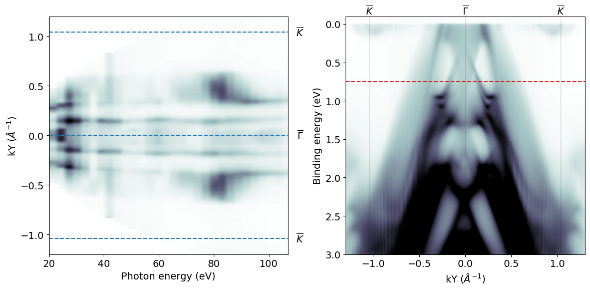
Plotting constant energy surfaces from hv-sweeps
Here we extract a constant energy surface, and beside it we plot the E-k image integrated over all photon energies. On that image we indicate where the energy surface is taken.
GK=1.041

hvscan = pesto.kwarp(pesto.loadSpectrum("snippets/PBT26New Region2026.ibw"))

# ---- Extract summation of all photon energies
hv_sum_image = pesto.getSlice(hvscan,axis=2,axisValue=66,sliceIntegration=999,beQuiet=True)

# ---- Extract constant binding energy slice
EbSlice=-0.75
eSurface = pesto.getSlice(hvscan,axis=0,axisValue=4.4-EbSlice,sliceIntegration=0.1,beQuiet=True)

fig,axis=plt.subplots(figsize=(12,6),ncols=2)

ax=axis[0]
pesto.quickPlot(eSurface,axis=ax)

#Optional - draw high symmetry lines
ax.axhline(y=0,ls='--')
ax.axhline(y=GK,ls='--')
ax.axhline(y=-GK,ls='--')

#Optional - label high symmetry lines
tform = matplotlib.transforms.blended_transform_factory(ax.transAxes,ax.transData)
ax.text(y=GK,x=1.05,s='$\overline{K}$',va='center', ha='center',transform=tform)
ax.text(y=-GK,x=1.05,s='$\overline{K}$',va='center', ha='center',transform=tform)
ax.text(y=0,x=1.05,s='$\overline{\Gamma}$',va='center', ha='center',transform=tform)

ax.set_ylim([-1.2,1.2])
ax.set_xlim([None,107])

ax=axis[1]
pesto.quickPlot(hv_sum_image,axis=ax,cmax=60000)
ax.set_ylim([3,-0.1])
ax.set_xlim([-1.3,1.3])
ax.axhline(y=-EbSlice,ls='--',color='tab:red')
highSymmetryPoints=[["$\overline{K}$",-GK],["$\overline{\Gamma}$",0],["$\overline{K}$",GK]]
pesto.drawHighSymmetryLabels(points=highSymmetryPoints,axis=ax)

plt.tight_layout()
plt.show()
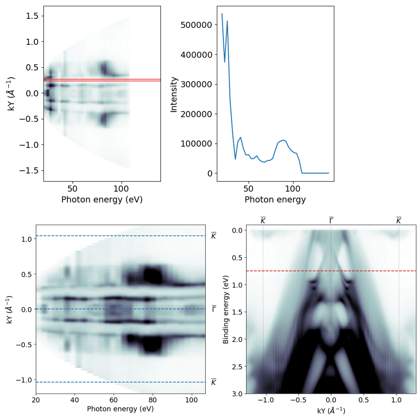
Sometimes for these scans it can be helpful to normalize. A simple approach to this is to pick a k region where the intensity is supposed to be uniform, and normalize to that. Here the first plot (which can be suppressed) shows in red where the normalization slice is taken:
GK=1.041

hvscan = pesto.kwarp(pesto.loadSpectrum("snippets/PBT26New Region2026.ibw"))

# ---- Extract summation of all photon energies
hv_sum_image = pesto.getSlice(hvscan,axis=2,axisValue=66,sliceIntegration=999,beQuiet=True)
# If the work function defined in SES is not correct, we'll need to shift the Eb scale to bring Ef up to zero

# ---- Extract constant binding energy slice
EbSlice=-0.75
eSurface = pesto.getSlice(hvscan,axis=0,axisValue=4.4-EbSlice,sliceIntegration=0.1,beQuiet=True)

# ---- Extract the line profile we will use for normalization
profile = pesto.getProfile(spectrum=eSurface,samplingAxis='x',yAxisRange=[0.24,0.27],xAxisRange=[0,999],beQuiet=False)
eSurface['dataNormalized']=np.zeros(np.shape(eSurface['data']))

for index,element in enumerate(profile['data']):
                                if element>0: eSurface['dataNormalized'][:,index]=[ii/element for ii in eSurface['data'][:,index]]
                                else: pass
eSurface['data']=eSurface['dataNormalized']


fig,axis=plt.subplots(figsize=(12,6),ncols=2)

ax=axis[0]
pesto.quickPlot(eSurface,axis=ax,cmax=0.25)

#Optional - draw high symmetry lines
ax.axhline(y=0,ls='--')
ax.axhline(y=GK,ls='--')
ax.axhline(y=-GK,ls='--')

#Optional - label high symmetry lines
tform = matplotlib.transforms.blended_transform_factory(ax.transAxes,ax.transData)
ax.text(y=GK,x=1.05,s='$\overline{K}$',va='center', ha='center',transform=tform)
ax.text(y=-GK,x=1.05,s='$\overline{K}$',va='center', ha='center',transform=tform)
ax.text(y=0,x=1.05,s='$\overline{\Gamma}$',va='center', ha='center',transform=tform)

ax.set_ylim([-1.2,1.2])
ax.set_xlim([None,107])

ax=axis[1]
pesto.quickPlot(hv_sum_image,axis=ax,cmax=60000)
ax.set_ylim([3,-0.1])
ax.set_xlim([-1.3,1.3])
ax.axhline(y=-EbSlice,ls='--',color='tab:red')
highSymmetryPoints=[["$\overline{K}$",-GK],["$\overline{\Gamma}$",0],["$\overline{K}$",GK]]
pesto.drawHighSymmetryLabels(points=highSymmetryPoints,axis=ax)

plt.tight_layout()
plt.show()
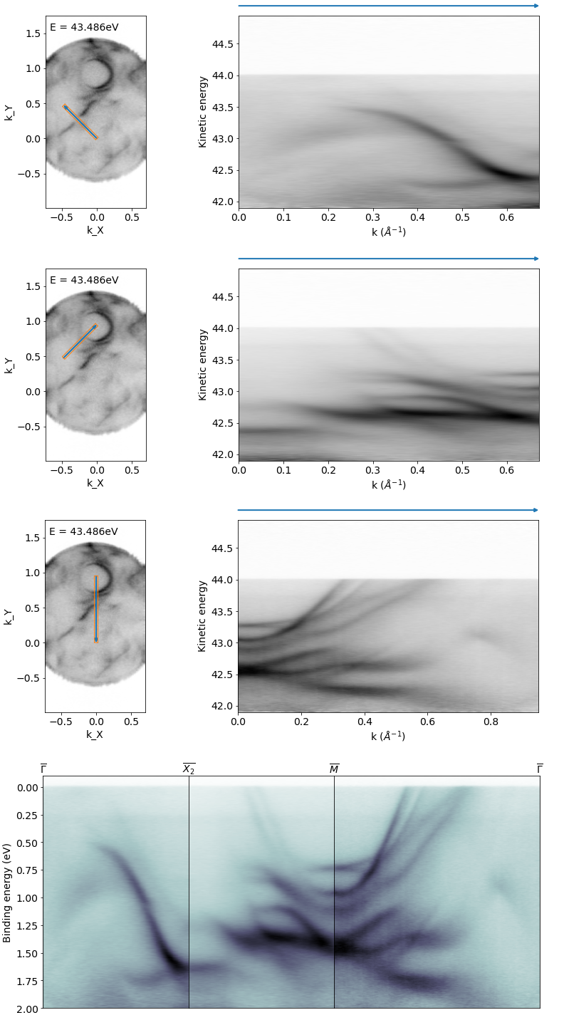
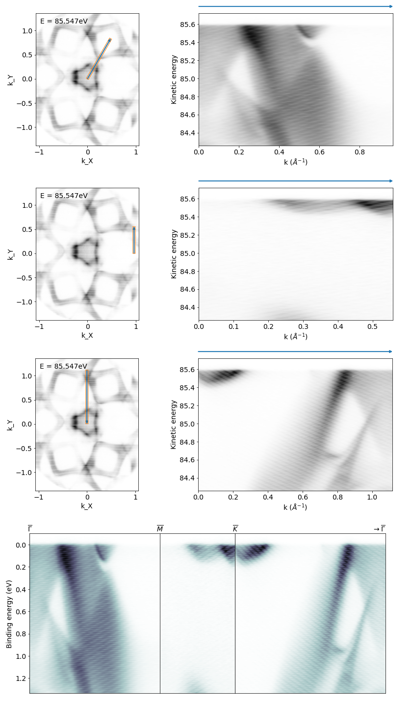
Extract arbitrary k-path from a 3D map
import matplotlib.gridspec as gridspec  #Needed for stacking images together
import math

# Define high symmetry points for the cuts to go to/from
# You may find it easier to just provide [kx,ky] coordinate pairs as read off from something like pesto.explorer
GM=0.952
GX=0.673
G = [0,0]
M = [0,GM]
X1=[GX/math.sqrt(2),GX/math.sqrt(2)]
X2=[-GX/math.sqrt(2),GX/math.sqrt(2)]

# Extract the cuts
hidePreviews=False
CII42_GX = pesto.getSliceArbitrary(spectrum = CII42_kwarped,startPoint=G,endPoint=X2,sliceIntegration=0.05,beQuiet=hidePreviews,previewEnergy=43.484)
CII42_XM=pesto.getSliceArbitrary(spectrum = CII42_kwarped,startPoint=X2,endPoint=M,sliceIntegration=0.05,beQuiet=hidePreviews,previewEnergy=43.484)
CII42_MG=pesto.getSliceArbitrary(spectrum = CII42_kwarped,startPoint=M,endPoint=G,sliceIntegration=0.05,beQuiet=hidePreviews,previewEnergy=43.484)

# Stack the cuts together side-by-side

hv = 48.75
fig = plt.figure(figsize=(12.5,6))
gs = gridspec.GridSpec(1, 3, width_ratios=[GX,GX,GM], height_ratios=[1])
gs.update(wspace = 0, hspace = 0)

ax = fig.add_subplot(gs[0])
pesto.quickPlot(CII42_GX,axis=ax,hv=hv)
ax.set_xticks([])
ax.set_ylim([2,-0.1])
ax.set_xlabel("")
highSymmetryPoints=[["$\overline{\Gamma}$",0]]
pesto.drawHighSymmetryLabels(points=highSymmetryPoints,axis=ax)

ax = fig.add_subplot(gs[1])
pesto.quickPlot(CII42_XM,axis=ax,hv=hv)
ax.set_ylabel("")
ax.set_xlabel("")
ax.set_xticks([])
ax.set_yticks([])
ax.set_ylim([2,-0.1])
highSymmetryPoints=[["$\overline{X_2}$",0]]
pesto.drawHighSymmetryLabels(points=highSymmetryPoints,axis=ax)

ax = fig.add_subplot(gs[2])
pesto.quickPlot(CII42_MG,axis=ax,hv=hv)
ax.set_ylabel("")
ax.set_xlabel("")
ax.set_xticks([])
ax.set_yticks([])
ax.set_ylim([2,-0.1])
highSymmetryPoints=[["$\overline{M}$",0],["$\overline{\Gamma}$",CII42_MG['Axis'][1][-1]]]
pesto.drawHighSymmetryLabels(points=highSymmetryPoints,axis=ax)
plt.show()
Here’s another example from a hexagonal symmetry sample:
import matplotlib.gridspec as gridspec

scan = pesto.loadSpectrum("example_data/PBT0007.zip",beQuiet=True)
scan_kwarped = pesto.kwarp(scan,beQuiet=True)

hv = 90.33
Ef = hv-pesto.ANALYZER_WORKFUNCTION

GM,GK,KM=0.967,1.117,0.559

G = [0,0]
M1 = [GM/2,(KM+(GK-KM)/2)]
M2 = [GM,0]
K1 = [GM,KM]
K2 = [0,GK]

# Extract the cuts
hidePreviews=False
PBT_GM = pesto.getSliceArbitrary(spectrum = scan_kwarped,startPoint=G,endPoint=M1,sliceIntegration=0.05,beQuiet=hidePreviews,previewEnergy=Ef-0.05)
PBT_MK = pesto.getSliceArbitrary(spectrum = scan_kwarped,startPoint=M2,endPoint=K1,sliceIntegration=0.05,beQuiet=hidePreviews,previewEnergy=Ef-0.05)
PBT_KG = pesto.getSliceArbitrary(spectrum = scan_kwarped,startPoint=K2,endPoint=G,sliceIntegration=0.05,beQuiet=hidePreviews,previewEnergy=Ef-0.05)

fig = plt.figure(figsize=(13,6))
gs = gridspec.GridSpec(1, 3, width_ratios=[GM,KM,GK], height_ratios=[1])
gs.update(wspace = 0, hspace = 0)

ax = fig.add_subplot(gs[0])
pesto.quickPlot(PBT_GM,axis=ax,hv=hv)
ax.set_xticks([])
ax.set_ylim([None,-0.1])
ax.set_xlabel("")
highSymmetryPoints=[["$\overline{\Gamma}$",0]]
pesto.drawHighSymmetryLabels(points=highSymmetryPoints,axis=ax)

ax = fig.add_subplot(gs[1])
pesto.quickPlot(PBT_MK,axis=ax,hv=hv)
ax.set_ylabel("")
ax.set_xlabel("")
ax.set_xticks([])
ax.set_yticks([])
ax.set_ylim([None,-0.1])
highSymmetryPoints=[["$\overline{M}$",0]]
pesto.drawHighSymmetryLabels(points=highSymmetryPoints,axis=ax)

ax = fig.add_subplot(gs[2])
pesto.quickPlot(PBT_KG,axis=ax,hv=hv)
ax.set_ylabel("")
ax.set_xlabel("")
ax.set_xticks([])
ax.set_yticks([])
ax.set_ylim([None,-0.1])
highSymmetryPoints=[["$\overline{K}$",0],["$\overline{\Gamma}$",scan_kwarped['Axis'][1][-1]]]
pesto.drawHighSymmetryLabels(points=highSymmetryPoints,axis=ax)
plt.show()
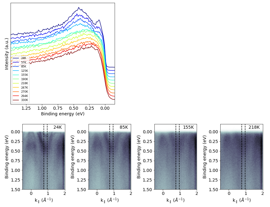
EDC series from a temperature dependence dataset
# Define what files to use and what temperatures they correspond to
fileIndices=[70,71,72,73,74,75,76,77,78,79,80]
temperatures=[24,57,85,125,155,190,218,247,270,294,330]
fileNames = ["example_data/FGT00{}Ek_1450{}.ibw".format(fileIndex,fileIndex) for fileIndex in fileIndices]

# Load them into memory
spectra = [pesto.kwarp(pesto.loadSpectrum(filename,regionIndex=1,beQuiet=True),tilt_offset=0.7,beQuiet=True) for filename in fileNames]

# Extract EDCs
hv = 145.33
centerK,kWidth = 0.86, 0.1
EbStart,EbEnd = 1.5, -0.2
EkStart = hv-pesto.ANALYZER_WORKFUNCTION-EbStart
EkEnd = hv-pesto.ANALYZER_WORKFUNCTION-EbEnd

EDCs=[pesto.getProfile(spectrum=spectrum,samplingAxis='y',xAxisRange=[centerK-kWidth,centerK+kWidth],yAxisRange=[EkStart,EkEnd],beQuiet=True) for spectrum in spectra]

# Normalize the EDCs to have the same value at high binding energy, and also apply an offset to space out the traces vertically
for index,EDC in enumerate(EDCs):
    EDC['data']-=min(EDC['data'])
    EDC['data']=EDC['data']/EDC['data'][0]
    EDC['data']=EDC['data']-(0.1*index)

# Plot EDC series
fig,ax = plt.subplots(figsize=[6,6])
ax.set_prop_cycle(plt.cycler('color', plt.cm.jet(np.linspace(0, 1, len(EDCs)))))

for spectrumIndex,EDC in enumerate(EDCs):
    pesto.quickPlot(EDC,axis=ax,hv=hv,lw=1.5,label="{}K".format(temperatures[spectrumIndex]))

ax.set_yticks([])
plt.legend(prop={'size': 9},loc='lower left')
plt.show()

# Plot a few E-k images showing where the EDCs are taken
fig,axes = plt.subplots(figsize=[12,4],ncols=4)
temperaturesToPlot=[24,85,155,218]
indicesToPlot = [pesto.indexOfClosestValue(temperatures,temperatureToPlot) for temperatureToPlot in temperaturesToPlot]

for axisIndex,spectrumIndex in enumerate(indicesToPlot):
    ax = axes[axisIndex]
    pesto.quickPlot(spectrum=spectra[spectrumIndex],axis=ax,hv=hv)
    ax.axvline(x=centerK+kWidth,color='black',ls='--')
    ax.axvline(x=centerK-kWidth,color='black',ls='--')
    ax.set_ylim([1.5,-0.2])
    ax.set_xlim([-0.5,2])
    ax.text(0.93, 0.93, "{}K".format(temperatures[spectrumIndex]), horizontalalignment='right', transform=ax.transAxes)
plt.tight_layout()
plt.show()
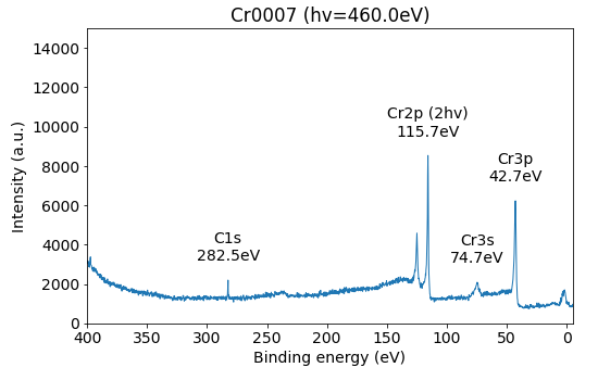
Labelled XPS spectra
This uses the ‘XPS=True’ argument of quickPlot to produce the plot, which collapses all angles down. The peak label function simply identifies the highest intensity within the range you have specified.
hv = 460

spectrum = pesto.loadSpectrum("example_data/Cr0007New Region1.ibw",beQuiet=True)
fig,ax=plt.subplots(figsize=(8,5))

pesto.quickPlot(spectrum,axis=ax,hv=hv,XPS=True)

ax.set_xlim([400,-5])
ax.set_ylim([0,1.5e4])

pesto.XPS.addPeakLabel(ax,spectrum,hv,xrange=[50,100],label='Cr3s')
pesto.XPS.addPeakLabel(ax,spectrum,hv,xrange=[250,290],label='C1s')
pesto.XPS.addPeakLabel(ax,spectrum,hv,xrange=[40,45],label='Cr3p')
pesto.XPS.addPeakLabel(ax,spectrum,hv,xrange=[100,120],label='Cr2p (2hv)')

ax.set_title("Cr0007 (hv={:.1f}eV)".format(hv))
plt.show()
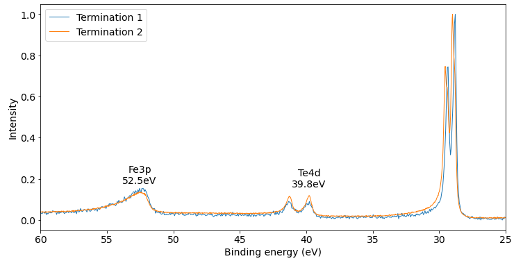
Compare multiple XPS spectra
Here we are comparing core levels from two different locations on the sample. The quickPlotXPS function is not suitable for more complicated operations like normalizing before plotting, so we need to collapse it down to a 1D trace ourselves with getProfile
scans=[]
scans.append(["Termination 1",pesto.loadSpectrum("example_data/FGT0052XPS_overview052.ibw",beQuiet=True)])
scans.append(["Termination 2",pesto.loadSpectrum("example_data/CII0045XPS_160eV045.ibw",beQuiet=True)])

hv = 160

fig,ax=plt.subplots(figsize=(8,5))

for scan in scans:
        label,spectrum = scan[0],scan[1]
        EDC = pesto.normalize(pesto.getProfile(spectrum=spectrum,samplingAxis='y',xAxisRange=[-15,15],yAxisRange=[0,999],beQuiet=True))
        pesto.quickPlot(EDC,axis=ax,hv=160,label=label)

ax.set_xlabel('Binding energy (eV)')
ax.set_ylabel('Intensity')
ax.legend()
ax.set_xlim([60,25])

pesto.XPS.addPeakLabel(axis=ax,spectrum=EDC,hv=hv,xrange=[50,60],label='Fe3p')
pesto.XPS.addPeakLabel(axis=ax,spectrum=EDC,hv=hv,xrange=[35,45],label='Te4d')

plt.show()
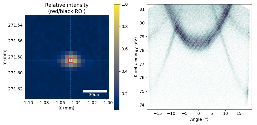
Contrast image from a spatial map
These code blocks are tedious to generate, so you would typically not do it by hand. Within pesto.explorer you have a button that will automatically generate this for you. After that you just need to make any minor formatting adjustments you like.
from mpl_toolkits.axes_grid1.anchored_artists import AnchoredSizeBar

spectrum=scan
scaleBarLength_um=30
point = [-1.045,271.585]
fig,axes=matplotlib.pyplot.subplots(figsize=(9,4),ncols=2)

ax=axes[1]
ROI_Angle,ROI_AngleIntegration = 3.772,1.93
ROI_Energy,ROI_EnergyIntegration = 78.649,0.38
ROI_AngleStart,ROI_AngleStop=ROI_Angle-ROI_AngleIntegration/2,ROI_Angle+ROI_AngleIntegration/2
ROI_EnergyStart,ROI_EnergyStop=ROI_Energy-ROI_EnergyIntegration/2,ROI_Energy+ROI_EnergyIntegration/2
ROI2_Angle,ROI2_AngleIntegration = 0.356,1.93
ROI2_Energy,ROI2_EnergyIntegration = 76.966,0.38
ROI2_AngleStart,ROI2_AngleStop=ROI2_Angle-ROI2_AngleIntegration/2,ROI2_Angle+ROI2_AngleIntegration/2
ROI2_EnergyStart,ROI2_EnergyStop=ROI2_Energy-ROI2_EnergyIntegration/2,ROI2_Energy+ROI2_EnergyIntegration/2

image = pesto.getFrameFrom4DScan(spectrum=spectrum,axes=['X','Y'],axisValues=point)
pesto.quickPlot(image,axis=ax)
ROI=matplotlib.patches.Rectangle((ROI_AngleStart,ROI_EnergyStart), height=ROI_EnergyIntegration, width=ROI_AngleIntegration,linestyle='-',color='tab:red',fill=False)
ax.add_patch(ROI)
ROI2=matplotlib.patches.Rectangle((ROI2_AngleStart,ROI2_EnergyStart), height=ROI2_EnergyIntegration, width=ROI2_AngleIntegration,linestyle='-',color='black',fill=False)
ax.add_patch(ROI2)
axes[0].set_title('Relative intensity (red/black ROI)')
map = pesto.spatialMap__RelativeIntensityContrastImage(spectrum,ROI_Angle,ROI_AngleIntegration,ROI_Energy,ROI_EnergyIntegration,ROI2_Angle,ROI2_AngleIntegration,ROI2_Energy,ROI2_EnergyIntegration)
ax=axes[0]
image=pesto.quickPlot(map,axis=ax,cmap='cividis',returnIm=True)
fig.colorbar(image,ax=ax)
x,y=point[0],point[1]
dx=abs(spectrum['Axis'][2][1]-spectrum['Axis'][2][0])
dy=abs(spectrum['Axis'][3][1]-spectrum['Axis'][3][0])
ax.axvline(x=x,ls='--')
ax.axhline(y=y,ls='--')
ROI=matplotlib.patches.Rectangle((x-(dx/2),y-(dy/2)), height=dy, width=dx,linestyle='-',color='tab:red',fill=False,lw=2)
ax.add_patch(ROI)

scalebar = AnchoredSizeBar(ax.transData,scaleBarLength_um/1000, '{}um'.format(scaleBarLength_um), 'lower right',pad=0.3,color='white',frameon=False,size_vertical=0.003)
ax.add_artist(scalebar)
plt.tight_layout()
plt.show()