spin module
These functions are specific to spin ARPES data from the B-endstation at Bloch. Consult the relevant blochdocs pages for discussion about what these calculations are doing and why.
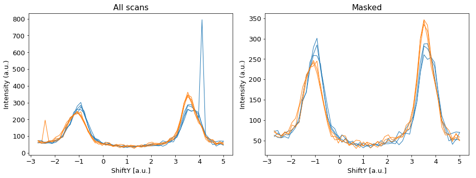
As a preliminary comment, don’t forget that you have the ‘mask’ argument available in pesto.loadSpectrum, which will allow you to ignore scans that have errors you can’t or don’t want to correct:
fig,axes=plt.subplots(figsize=[13,5],ncols=2)

spinScan = pesto.loadSpectrum("example_data/spinMDC/id34_C2_r+.xy",beQuiet=True)
ax=axes[0]
ax.set_title("All scans")
for ii,scanIndex in enumerate(spinScan['Axis'][1]):
    EDC = pesto.getProfile(spinScan,samplingAxis='y',xAxisRange=[scanIndex,scanIndex],beQuiet=True)
    if spinScan['Metadata']['CoilPolarity'][ii]=='Positive': color='tab:blue'
    else: color='tab:orange'
    pesto.quickPlot(EDC,axis=ax,color=color)

spinScan = pesto.loadSpectrum("example_data/spinMDC/id34_C2_r+.xy",beQuiet=True,mask=[1,1,1,0,1,1,0,1])

ax=axes[1]
ax.set_title("Masked")

for ii,scanIndex in enumerate(spinScan['Axis'][1]):
    EDC = pesto.getProfile(spinScan,samplingAxis='y',xAxisRange=[scanIndex,scanIndex],beQuiet=True)
    if spinScan['Metadata']['CoilPolarity'][ii]=='Positive': color='tab:blue'
    else: color='tab:orange'
    pesto.quickPlot(EDC,axis=ax,color=color)

plt.tight_layout()
plt.show()
spin.despike
Removes spurious intensity spikes in spin measurements. It first calculates the median value and the spread in values (i.e. abs(max-min)) at each scanpoint (energy or angle) for the positive and negative polarity scan sets. It then proceeds point-by-point through each individual scan, and if it finds a datapoint that is outside of the window (median +/- (spread/2)*tolerance), it replaces the offending datapoint with NaN.
Since it is not a-priori obvious what the optimal tolerance value is for the filtering, by default this launches as an interactive widget. It works for both 1D and 2D spin spectra.
def spin.despike(spectrum,interactive,toleranceFactor)
Required parameters
spectrum: a pesto spectrum that contains a single spin-EDC or spin-MDC profile, or a 2D spin-image, repeated for multiple different target magnetizations.
Optional parameters
interactive: If true, brings up an interactive widget to allow you to determine the optimal value for toleranceFactor. If you already know this value, setting interactive=False will perform the operation quietly in the background and return a new, despiked copy of the input spectrum. Default = True
toleranceFactor: How far a datapoint is allowed to be outside the ‘normal’ range of values before it gets assigned NaN. Default = 1
- Returns:
A new pesto spectrum dictionary if interactive=False, else an interactive widget.
Example usage:


spin.sumProfiles
def spin.sumProfiles(spectrum)
Required parameters
spectrum: a pesto spectrum that contains a single spin-EDC or spin-MDC profile, repeated for multiple different target magnetizations.
- Returns:
Two new pesto spectrum dictionaries (one for each target magnetization) that each contain just a single summed 1D dataset
Example usage:
spinScan = pesto.loadSpectrum("example_data/spinMDC/id34_C2_r+.xy",beQuiet=True,mask=[1,1,1,0,1,1,0,1])

fig,axes=plt.subplots(figsize=[13,5],ncols=2)
ax=axes[0]
ax.set_title("All scans")
for ii,scanIndex in enumerate(spinScan['Axis'][1]):
    EDC = pesto.getProfile(spinScan,samplingAxis='y',xAxisRange=[scanIndex,scanIndex],beQuiet=True)
    if spinScan['Metadata']['CoilPolarity'][ii]=='Positive': color='tab:blue'
    else: color='tab:orange'
    pesto.quickPlot(EDC,axis=ax,color=color)

ax=axes[1]
ax.set_title("Summed")

targetPlus,targetMinus = pesto.spin.sumProfiles(spinScan)

pesto.quickPlot(targetPlus,axis=ax,label="Coil polarity +")
pesto.quickPlot(targetMinus,axis=ax,label="Coil polarity -")
ax.legend()
plt.tight_layout()
plt.show()
spin.calculateAverageProfiles
Identical to sumProfiles, except that it returns the average profiles.
def spin.calculateAverageProfiles(spectrum)
Required parameters
spectrum: a pesto spectrum that contains a single spin-EDC or spin-MDC profile, repeated for multiple different target magnetizations.
- Returns:
Two new pesto spectrum dictionaries (one for each target magnetization) that each contain just a single averaged 1D dataset
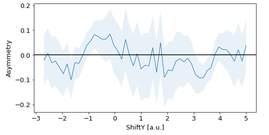
spin.calculateAsymmetry
def spin.calculateAsymmetry(spectrum)
Required parameters
spectrum: a pesto spectrum that contains a single spin-EDC or spin-MDC profile, repeated for multiple different target magnetizations.
- Returns:
A new pesto spectrum dictionary containing the averaged asymmetry of the input spectrum. The error bars are included in the [‘error’] field
Example usage:
spinScan = pesto.loadSpectrum("example_data/spinMDC/id34_C2_r+.xy",beQuiet=True)

fig,ax=plt.subplots(figsize=[8,4])

asymmetry = pesto.spin.calculateAsymmetry(spinScan)

pesto.quickPlot(asymmetry,errorbars=True,axis=ax)
ax.axhline(y=0,color='black')
ax.set_ylabel("Asymmetry")
plt.show()
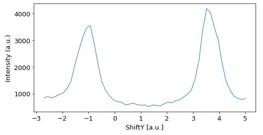
spin.calculateIntegratedIntensity
Given a list of spin spectra, this will return the total intensity, combining both coil polarities. This is useful for computing spin-resolved component spectra, and also for cross-referencing measurements with a spin-integrated CCD measurement.
def calculateIntegratedIntensity(spectra)
Parameters
spectra: A list of pesto spectra (or filenames) that contain single spin-EDC or spin-MDC profiles. All inputs must have the same scan range and step size.
- Returns:
A new pesto spectrum dictionary containing the sum of all profiles in the input spectra. The error bars are included in the [‘error’] field
Example usage:
c2rp=pesto.loadSpectrum("example_data/spinMDC/id34_C2_r+.xy",beQuiet=True,mask=[1,1,1,0,1,1,0,1])
c2rm=pesto.loadSpectrum("example_data/spinMDC/id35_C2_r-.xy",beQuiet=True)

sumIntensity = pesto.spin.calculateIntegratedIntensity(scans=[c2rp,c2rm])

fig,ax=plt.subplots(figsize=[8,4])
pesto.quickPlot(sumIntensity,axis=ax)
plt.show()
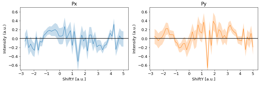
spin.calculatePolarization
Given 1-3 sets of 1D spin profiles (corresponding to different rotator or coil polarity settings), this function will return whatever polarization information is possible to deduce. Two datasets are required to obtain the Px and Py components (coil2 rotator+, coil2 rotator-), while a third is required to obtain the Pz components (coil 1).
def spin.calculateAsymmetry(  c2rp,
                              c2rm,
                              c1,
                              sherman)
Required Parameters
Technically none, but to get any meaningful output you need either (c2rp + c2rm), c1, or all three.
Optional parameters
c2rp: a pesto spectrum (or filename) that contains a single spin-EDC or spin-MDC profile, repeated for multiple different target magnetizations, with the specific configuration of spin rotator +, target magnetized with coil 2. Default = None
c2rm: a pesto spectrum (or filename) that contains a single spin-EDC or spin-MDC profile, repeated for multiple different target magnetizations, with the specific configuration of spin rotator -, target magnetized with coil 2. Default = None
c1: a pesto spectrum (or filename) that contains a single spin-EDC or spin-MDC profile, repeated for multiple different target magnetizations, with the specific configuration of target magnetized with coil 1 (any rotator setting). Default = None
sherman: Sherman function to use. Default = 0.29
- Returns:
Px,Py,Pz spectra, including error bars. If not enough input data was provided, some or all of these will be None instead of a valid pesto spectrum.
Example usage:
c2rp=pesto.loadSpectrum("example_data/spinMDC/id34_C2_r+.xy",beQuiet=True,mask=[1,1,1,0,1,1,0,1])
c2rm=pesto.loadSpectrum("example_data/spinMDC/id35_C2_r-.xy",beQuiet=True)

px,py,pz = pesto.spin.calculatePolarization(c2rp=c2rp,c2rm=c2rm)

fig,axes=plt.subplots(figsize=[12,4],ncols=2)

ax=axes[0]
pesto.quickPlot(px,errorbars=True,axis=ax,alpha=0.25)
ax.axhline(y=0,color='black')
ax.set_ylim([-0.7,0.7])
ax.set_title("Px")

ax=axes[1]
pesto.quickPlot(py,errorbars=True,axis=ax,color='tab:orange',alpha=0.25)
ax.axhline(y=0,color='black')
ax.set_title("Py")
ax.set_ylim([-0.7,0.7])

plt.tight_layout()
plt.show()
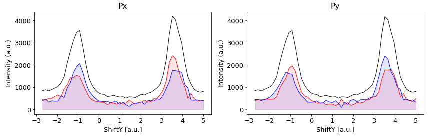
spin.calculateComponentIntensity
Given 1-3 sets of 1D spin profiles (corresponding to different rotator or coil polarity settings), this function will return whatever component intensity information is possible to deduce. Two datasets are required to obtain the Px and Py components (coil2 rotator+, coil2 rotator-), while a third is required to obtain the Pz components (coil 1).
def spin.calculateComponentIntensity( c2rp,
                                      c2rm,
                                      c1,
                                      sherman)
Required Parameters
Technically none, but to get any meaningful output you need either (c2rp + c2rm), c1, or all three.
Optional parameters
c2rp: a pesto spectrum (or filename) that contains a single spin-EDC or spin-MDC profile, repeated for multiple different target magnetizations, with the specific configuration of spin rotator +, target magnetized with coil 2. Default = None
c2rm: a pesto spectrum (or filename) that contains a single spin-EDC or spin-MDC profile, repeated for multiple different target magnetizations, with the specific configuration of spin rotator -, target magnetized with coil 2. Default = None
c1: a pesto spectrum (or filename) that contains a single spin-EDC or spin-MDC profile, repeated for multiple different target magnetizations, with the specific configuration of target magnetized with coil 1 (any rotator setting). Default = None
sherman: Sherman function to use. Default = 0.29
- Returns:
Px_plus,Px_minus,Py_plus,Py_minus,Pz_plus,Pz_minus spectra, currently not including error bars. If not enough input data was provided, some or all of these will be None instead of a valid pesto spectrum.
Example usage:
c2rp=pesto.loadSpectrum("example_data/spinMDC/id34_C2_r+.xy",beQuiet=True,mask=[1,1,1,0,1,1,0,1])
c2rm=pesto.loadSpectrum("example_data/spinMDC/id35_C2_r-.xy",beQuiet=True)

xp,xm,yp,ym,zp,zm = pesto.spin.calculateComponentIntensity(c2rp=c2rp,c2rm=c2rm)
sumIntensity = pesto.spin.calculateIntegratedIntensity(scans=[c2rp,c2rm])

fig,axes=plt.subplots(figsize=[12,4],ncols=2)
ax=axes[0]
pesto.quickPlot(xp,axis=ax,filled=True,color='red')
pesto.quickPlot(xm,axis=ax,filled=True,color='blue')
pesto.quickPlot(sumIntensity,axis=ax,color='black')
ax.set_title("Px")
ax=axes[1]
pesto.quickPlot(yp,axis=ax,filled=True,color='red',alpha=0.1)
pesto.quickPlot(ym,axis=ax,filled=True,color='blue',alpha=0.1)
pesto.quickPlot(sumIntensity,axis=ax,color='black')
ax.set_title("Py")
plt.tight_layout()
plt.show()
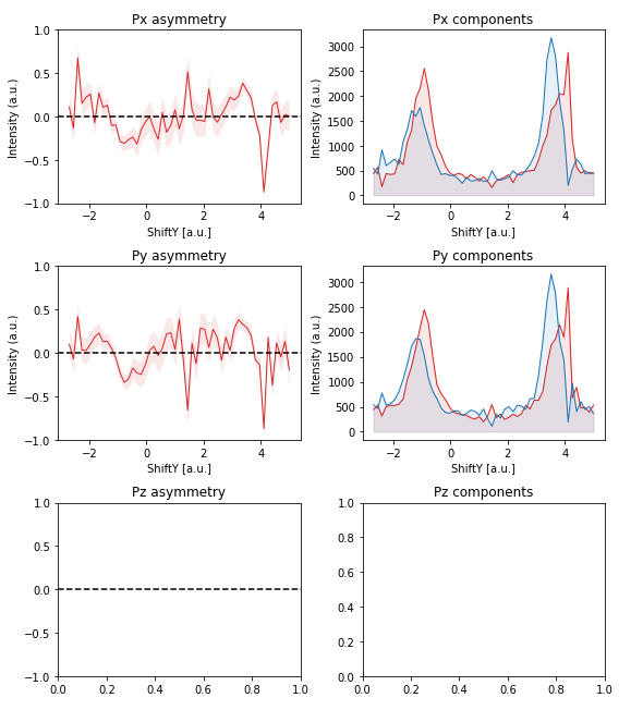
spin.quickSummary
Given 1-3 sets of 1D spin profiles (corresponding to different rotator or coil polarity settings), this function will produces a summary plot of asymmetry and spin-resolved components.
def spin.quickSummary(  c2rp,
                        c2rm,
                        c1)
Required Parameters
Technically none, but to get any meaningful output you need either (c2rp + c2rm), c1, or all three.
Optional parameters
c2rp: a pesto spectrum (or filename) that contains a single spin-EDC or spin-MDC profile, repeated for multiple different target magnetizations, with the specific configuration of spin rotator +, target magnetized with coil 2. Default = None
c2rm: a pesto spectrum (or filename) that contains a single spin-EDC or spin-MDC profile, repeated for multiple different target magnetizations, with the specific configuration of spin rotator -, target magnetized with coil 2. Default = None
c1: a pesto spectrum (or filename) that contains a single spin-EDC or spin-MDC profile, repeated for multiple different target magnetizations, with the specific configuration of target magnetized with coil 1 (any rotator setting). Default = None
- Returns:
Nothing (prints a summary plot)
Example usage:
pesto.spin.quickSummary(c2rm="example_data/spinMDC/id34_C2_r+.xy",c2rp="example_data/spinMDC/id35_C2_r-.xy")